More Examples

At this point it would be wise to begin familiarizing yourself more systematically with PyTensor’s fundamental objects and operations by browsing this section of the library: Basic Tensor Functionality.

As the tutorial unfolds, you should also gradually acquaint yourself with the other relevant areas of the library and with the relevant subjects of the documentation entrance page.

Logistic Function

Here’s another straightforward example, though a bit more elaborate than adding two numbers together. Let’s say that you want to compute the logistic curve, which is given by:

\[s(x) = \frac{1}{1 + e^{-x}}\]

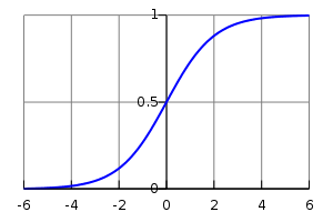
A plot of the logistic function, with \(x\) on the x-axis and \(s(x)\) on the y-axis.

You want to compute the function element-wise on matrices of doubles, which means that you want to apply this function to each individual element of the matrix.

Well, what you do is this:

>>> import pytensor
>>> import pytensor.tensor as pt
>>> x = pt.dmatrix('x')
>>> s = 1 / (1 + pt.exp(-x))
>>> logistic = pytensor.function([x], s)
>>> logistic([[0, 1], [-1, -2]])
array([[0.5       , 0.73105858],
       [0.26894142, 0.11920292]])

The reason the logistic is applied element-wise is because all of its operations–division, addition, exponentiation, and division–are themselves element-wise operations.

It is also the case that:

\[s(x) = \frac{1}{1 + e^{-x}} = \frac{1 + \tanh(x/2)}{2}\]

We can verify that this alternate form produces the same values:

>>> s2 = (1 + pt.tanh(x / 2)) / 2
>>> logistic2 = pytensor.function([x], s2)
>>> logistic2([[0, 1], [-1, -2]])
array([[0.5       , 0.73105858],
       [0.26894142, 0.11920292]])

Computing More than one Thing at the Same Time

PyTensor supports functions with multiple outputs. For example, we can compute the element-wise difference, absolute difference, and squared difference between two matrices a and b at the same time:

>>> a, b = pt.dmatrices('a', 'b')
>>> diff = a - b
>>> abs_diff = abs(diff)
>>> diff_squared = diff**2
>>> f = pytensor.function([a, b], [diff, abs_diff, diff_squared])

Note

dmatrices produces as many outputs as names that you provide. It is a shortcut for allocating symbolic variables that we will often use in the tutorials.

When we use the function f, it returns the three variables (the printing was reformatted for readability):

>>> f([[1, 1], [1, 1]], [[0, 1], [2, 3]])
[array([[ 1.,  0.],
       [-1., -2.]]), array([[1., 0.],
       [1., 2.]]), array([[1., 0.],
       [1., 4.]])]

Setting a Default Value for an Argument

Let’s say you want to define a function that adds two numbers, except that if you only provide one number, the other input is assumed to be one. You can do it like this:

>>> from pytensor.compile.io import In
>>> from pytensor import function
>>> x, y = pt.dscalars('x', 'y')
>>> z = x + y
>>> f = function([x, In(y, value=1)], z)
>>> f(33)
array(34.)
>>> f(33, 2)
array(35.)

This makes use of the In class which allows you to specify properties of your function’s parameters with greater detail. Here we give a default value of 1 for y by creating a In instance with its value field set to 1.

Inputs with default values must follow inputs without default values (like Python’s functions). There can be multiple inputs with default values. These parameters can be set positionally or by name, as in standard Python:

>>> x, y, w = pt.dscalars('x', 'y', 'w')
>>> z = (x + y) * w
>>> f = function([x, In(y, value=1), In(w, value=2, name='w_by_name')], z)
>>> f(33)
array(68.)
>>> f(33, 2)
array(70.)
>>> f(33, 0, 1)
array(33.)
>>> f(33, w_by_name=1)
array(34.)
>>> f(33, w_by_name=1, y=0)
array(33.)

Note

In does not know the name of the local variables y and w that are passed as arguments. The symbolic variable objects have name attributes (set by dscalars in the example above) and these are the names of the keyword parameters in the functions that we build. This is the mechanism at work in In(y, value=1). In the case of In(w, value=2, name='w_by_name'). We override the symbolic variable’s name attribute with a name to be used for this function.

You may like to see Function in the library for more detail.

Using Shared Variables

It is also possible to make a function with an internal state. For example, let’s say we want to make an accumulator: at the beginning, the state is initialized to zero, then, on each function call, the state is incremented by the function’s argument.

First let’s define the accumulator function. It adds its argument to the internal state and returns the old state value.

>>> from pytensor import shared
>>> state = shared(0)
>>> inc = pt.iscalar('inc')
>>> accumulator = function([inc], state, updates=[(state, state+inc)])

This code introduces a few new concepts. The shared function constructs so-called shared variables. These are hybrid symbolic and non-symbolic variables whose value may be shared between multiple functions. Shared variables can be used in symbolic expressions just like the objects returned by dmatrices but they also have an internal value that defines the value taken by this symbolic variable in all the functions that use it. It is called a shared variable because its value is shared between many functions. The value can be accessed and modified by the get_value() and set_value() methods. We will come back to this soon.

The other new thing in this code is the updates parameter of pytensor.function(). updates must be supplied with a list of pairs of the form (shared-variable, new expression). It can also be a dictionary whose keys are shared-variables and values are the new expressions. Either way, it means “whenever this function runs, it will replace the value of each shared variable with the result of the corresponding expression”. Above, our accumulator replaces the state’s value with the sum of the state and the increment amount.

Let’s try it out!

>>> print(state.get_value())
0
>>> accumulator(1)
array(0)
>>> print(state.get_value())
1
>>> accumulator(300)
array(1)
>>> print(state.get_value())
301

It is possible to reset the state. Just use the .set_value() method:

>>> state.set_value(-1)
>>> accumulator(3)
array(-1)
>>> print(state.get_value())
2

As we mentioned above, you can define more than one function to use the same shared variable. These functions can all update the value.

>>> decrementor = function([inc], state, updates=[(state, state-inc)])
>>> decrementor(2)
array(2)
>>> print(state.get_value())
0

You might be wondering why the updates mechanism exists. You can always achieve a similar result by returning the new expressions, and working with them in NumPy as usual. The updates mechanism can be a syntactic convenience, but it is mainly there for efficiency. Updates to shared variables can sometimes be done more quickly using in-place algorithms (e.g. low-rank matrix updates).

It may happen that you expressed some formula using a shared variable, but you do not want to use its value. In this case, you can use the givens parameter of pytensor.function() which replaces a particular node in a graph for the purpose of one particular function.

>>> fn_of_state = state * 2 + inc
>>> # The type of foo must match the shared variable we are replacing
>>> # with the ``givens``
>>> foo = pt.scalar(dtype=state.dtype)
>>> skip_shared = function([inc, foo], fn_of_state, givens=[(state, foo)])
>>> skip_shared(1, 3)  # we're using 3 for the state, not state.value
array(7)
>>> print(state.get_value())  # old state still there, but we didn't use it
0

The givens parameter can be used to replace any symbolic variable, not just a shared variable. You can replace constants, and expressions, in general. Be careful though, not to allow the expressions introduced by a givens substitution to be co-dependent, the order of substitution is not defined, so the substitutions have to work in any order.

In practice, a good way of thinking about the givens is as a mechanism that allows you to replace any part of your formula with a different expression that evaluates to a tensor of same shape and dtype.

Note

PyTensor shared variable broadcast pattern default to False for each dimensions. Shared variable size can change over time, so we can’t use the shape to find the broadcastable pattern. If you want a different pattern, just pass it as a parameter pytensor.shared(..., broadcastable=(True, False))

Note

Use the shape parameter to specify tuples of static shapes instead; the old broadcastable values are being phased-out. Unknown shape values for dimensions take the value None; otherwise, integers are used for known static shape values. For example, pytensor.shared(..., shape=(1, None)).

Copying functions

PyTensor functions can be copied, which can be useful for creating similar functions but with different shared variables or updates. This is done using the pytensor.compile.executor.Function.copy() method of Function objects. The optimized graph of the original function is copied, so compilation only needs to be performed once.

Let’s start from the accumulator defined above:

>>> import pytensor
>>> import pytensor.tensor as pt
>>> state = pytensor.shared(0)
>>> inc = pt.iscalar('inc')
>>> accumulator = pytensor.function([inc], state, updates=[(state, state+inc)])

We can use it to increment the state as usual:

>>> accumulator(10)
array(0)
>>> print(state.get_value())
10

We can use copy() to create a similar accumulator but with its own internal state using the swap parameter, which is a dictionary of shared variables to exchange:

>>> new_state = pytensor.shared(0)
>>> new_accumulator = accumulator.copy(swap={state:new_state})
>>> new_accumulator(100)
array(0)
>>> print(new_state.get_value())
100

The state of the first function is left untouched:

>>> print(state.get_value())
10

We now create a copy with updates removed using the delete_updates parameter, which is set to False by default:

>>> null_accumulator = accumulator.copy(delete_updates=True)

As expected, the shared state is no longer updated:

>>> null_accumulator(9000)
array(10)
>>> print(state.get_value())
10

Using Random Numbers

Because in PyTensor you first express everything symbolically and afterwards compile this expression to get functions, using pseudo-random numbers is not as straightforward as it is in NumPy, though also not too complicated.

The API is documented in pytensor.tensor.random. For a more technical explanation of how PyTensor implements random variables see Pseudo random number generation in PyTensor.

Brief Example

Here’s a brief example. We create a shared RNG, draw from two distributions, and compile a function with update rules so the RNG state advances between calls:

import numpy as np
import pytensor
import pytensor.tensor as pt

rng = pt.random.shared_rng(seed=123)
next_rng, rv_u = rng.uniform(0, 1, size=(2, 2))
final_rng, rv_n = next_rng.normal(0, 1, size=(2, 2))

f = pytensor.function([], [rv_u, rv_n], updates={rng: final_rng})

Here, rv_u represents a 2x2 matrix of draws from a uniform distribution and rv_n a 2x2 matrix of draws from a normal distribution. Note how we thread next_rng into the second draw to ensure each gets a different RNG state. The updates dictionary tells the function to update the shared RNG with the final state after each call, so subsequent calls produce different numbers.

Reseeding

You can reseed a shared RNG by setting its value to a fresh generator or seed:

rng.set_value(np.random.default_rng(42))
# Or equivalently
rng.set_value(seed=42)

This resets the RNG state so subsequent calls to f() will produce a new deterministic sequence.

Other Random Distributions

There are many distributions available as methods on RNG variables (e.g. rng.normal(), rng.uniform()).

A Real Example: Logistic Regression

The preceding elements are featured in this more realistic example. It will be used repeatedly.

import numpy as np
import pytensor
import pytensor.tensor as pt


rng = np.random.default_rng(2882)

N = 400                                   # training sample size
feats = 784                               # number of input variables

# generate a dataset: D = (input_values, target_class)
D = (rng.standard_normal((N, feats)), rng.integers(size=N, low=0, high=2))
training_steps = 10000

# Declare PyTensor symbolic variables
x = pt.dmatrix("x")
y = pt.dvector("y")

# initialize the weight vector w randomly
#
# this and the following bias variable b
# are shared so they keep their values
# between training iterations (updates)
w = pytensor.shared(rng.standard_normal(feats), name="w")

# initialize the bias term
b = pytensor.shared(0., name="b")

print("Initial model:")
print(w.get_value())
print(b.get_value())

# Construct PyTensor expression graph
p_1 = 1 / (1 + pt.exp(-pt.dot(x, w) - b))       # Probability that target = 1
prediction = p_1 > 0.5                          # The prediction thresholded
xent = -y * pt.log(p_1) - (1-y) * pt.log(1-p_1) # Cross-entropy loss function
cost = xent.mean() + 0.01 * (w ** 2).sum()      # The cost to minimize
gw, gb = pt.grad(cost, [w, b])                  # Compute the gradient of the cost
                                                # w.r.t weight vector w and
                                                # bias term b (we shall
                                                # return to this in a
                                                # following section of this
                                                # tutorial)

# Compile
train = pytensor.function(
          inputs=[x,y],
          outputs=[prediction, xent],
          updates=((w, w - 0.1 * gw), (b, b - 0.1 * gb)))
predict = pytensor.function(inputs=[x], outputs=prediction)

# Train
for i in range(training_steps):
    pred, err = train(D[0], D[1])

print("Final model:")
print(w.get_value())
print(b.get_value())
print("target values for D:")
print(D[1])
print("prediction on D:")
print(predict(D[0]))